Modelling interactions • kagu

In traditional linear modelling (lm), interactions between variables must be explicitly specified by the researcher (e.g., y ~ a * b). If you forget to include the interaction term, the model is forced to assume that the effect of a is strictly independent of b, leading to biased or incomplete estimates.

Kagu takes a different approach. Because Kagu models each node as a Gaussian Process over an eigen-basis of its parents, interactions are learned automatically. The GP naturally spans the multi-dimensional surface of its inputs, capturing non-linearities and interactions without any explicit formula from the user.

In this vignette, we’ll look at how to recover and visualise a continuous-continuous interaction using Kagu’s effect estimation.

A system with a strong interaction

Let’s simulate a system where $A$ and $B$ are independent causes of $Y$ , but they interact multiplicatively. The true data-generating process is: $Y = 1.5 A - 1.0 B + 2.0 (A \times B) + \epsilon$

Because of the positive $2.0$ interaction term, the effect of $A$ on $Y$ heavily depends on the value of $B$ . If $B$ is positive, $A$ has a strong positive effect. If $B$ is negative, $A$ ’s effect might even become negative!

n <- 500
a <- rnorm(n)
b <- rnorm(n)
y <- 1.5 * a - 1.0 * b + 2.0 * (a * b) + rnorm(n, sd = 0.5)

df <- data.frame(a, b, y)

We define our Kagu model as usual and fit it. Notice that we do not tell Kagu about the interaction.

dag <- list(
  a = c(),
  b = c(),
  y = c("a", "b")
)

mod <- KaguModel$new(dag)
mod$fit(df)

The marginal effect

If we ask Kagu for the effect of a on y without specifying anything else, it integrates out the uncertainty and natural distribution of b over the dataset.

# The average marginal gradient of a -> y
mod$effects("a", "y")$summary()
#> # A tibble: 1 × 8
#>   source target    from    to  mean    sd hdi_lower hdi_upper
#>   <chr>  <chr>    <dbl> <dbl> <dbl> <dbl>     <dbl>     <dbl>
#> 1 a      y      -0.0300 0.970  1.41 0.108      1.25      1.59

The average effect is positive (around 1.5), which matches the main effect of a in our simulation. However, the standard deviation/HDI is quite wide. That’s because the “true” effect of a is not a single number-it’s highly variable depending on b.

Conditioning to reveal the interaction

To probe the interaction, we can estimate the effect of a on y while conditioning b at specific values using the conditions argument.

Let’s look at the gradient (the local slope) of a -> y when $B = -1$ , $B = 0$ , and $B = 1$ :

# Slope when b = -1
mod$effects("a", "y", conditions = list(b = -1))$summary()
#> # A tibble: 1 × 8
#>   source target    from    to   mean     sd hdi_lower hdi_upper
#>   <chr>  <chr>    <dbl> <dbl>  <dbl>  <dbl>     <dbl>     <dbl>
#> 1 a      y      -0.0300 0.970 -0.621 0.0526    -0.709    -0.537

# Slope when b = 0
mod$effects("a", "y", conditions = list(b = 0))$summary()
#> # A tibble: 1 × 8
#>   source target    from    to  mean     sd hdi_lower hdi_upper
#>   <chr>  <chr>    <dbl> <dbl> <dbl>  <dbl>     <dbl>     <dbl>
#> 1 a      y      -0.0300 0.970  1.46 0.0437      1.39      1.53

# Slope when b = 1
mod$effects("a", "y", conditions = list(b = 1))$summary()
#> # A tibble: 1 × 8
#>   source target    from    to  mean     sd hdi_lower hdi_upper
#>   <chr>  <chr>    <dbl> <dbl> <dbl>  <dbl>     <dbl>     <dbl>
#> 1 a      y      -0.0300 0.970  3.59 0.0466      3.52      3.68

The model successfully recovered the interaction! * At $B = -1$ , the expected slope is $1.5 + 2.0(-1) = -0.5$ . Kagu estimates $\approx -0.5$ . * At $B = 0$ , the expected slope is $1.5 + 2.0(0) = 1.5$ . Kagu estimates $\approx 1.5$ . * At $B = 1$ , the expected slope is $1.5 + 2.0(1) = 3.5$ . Kagu estimates $\approx 3.5$ .

Visualising the interaction with sweeps

We can visualise this interactive surface by requesting sweep = TRUE. Rather than computing the effects one at a time and combining them manually, we can pass a list of conditions directly to $effects().

Kagu will automatically compute the sweep under each condition, bundle them together, and overlay them seamlessly when you call $plot()!

# Request full sweeps of a -> y at different levels of b
eff_multi <- mod$effects("a", "y", sweep = TRUE, conditions = list(
  list(b = -1),
  list(b = 0),
  list(b = 1)
))

# Plot the interaction seamlessly
eff_multi$plot() +
  scale_color_manual(values = c("b=-1" = "#ff7043", "b=0" = "#9e9e9e", "b=1" = "#26a69a")) +
  scale_fill_manual(values = c("b=-1" = "#ff7043", "b=0" = "#9e9e9e", "b=1" = "#26a69a")) +
  ggtitle("Continuous-Continuous Interaction: a -> y conditioned on b")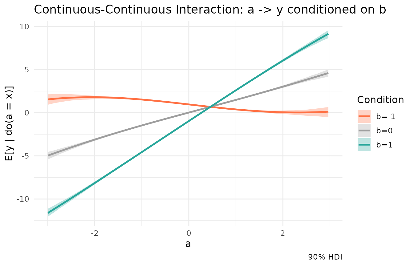

The diverging slopes clearly show the interaction effect.

By treating causal mechanisms as flexible Gaussian Processes, Kagu frees you from having to guess or pre-specify the exact functional form of your causal relationships. Interactions are automatically detected, naturally accommodated, and easily visualised using the conditions argument!