Case study: Sociality and fitness in ecology • kagu

In this vignette, we explore a classic observational study in behavioural ecology. We’ll use Kagu to perform causal discovery, estimate effects, unmask hidden interactions, and avoid the notorious “Table II fallacy” common in traditional regression.

The study system

Imagine a long-term field study of a social mammal population (e.g., macaques, dolphins, or elephants). We have collected observational data on 50 individuals - a small, noisy field dataset typical of hard-to-observe wild populations - measuring five variables:

age: Age of the individual (standardised).
sex: Female (-1) or Male (1).
sociality: A continuous index of social network centrality.
food_sharing: The rate at which the individual participates in cooperative food sharing.
condition: Body condition index (e.g., girth-to-length ratio; a proxy for fitness).

The true causal structure

We simulate the data based on expert domain knowledge of the species:

Age $\to$ Sociality: Older individuals have had more time to establish social bonds.
Age $\to$ Condition: Older individuals are more experienced foragers, directly improving their condition independent of sociality. This makes age a confounder of the sociality-condition relationship.
Sociality $\to$ Food sharing: More central individuals share food more often.
Food sharing $\to$ Condition: Receiving shared food directly improves caloric intake and body condition. This makes food_sharing a mediator on the path from sociality to condition.
Sex $\to$ Condition: Males and females differ in baseline condition due to sexual dimorphism.
Sociality $\to$ Condition (Direct, interacting with Sex): Sociality also directly affects condition through stress buffering (e.g., lower cortisol). However, this effect is highly sex-dependent. For females, sociality means allomaternal support and reduced stress (positive effect). For males, sociality means proximity to competitors and higher agonistic stress (negative effect).

Let’s simulate 50 individuals from this exact process:

n <- 50
sex <- sample(c(-1, 1), n, replace = TRUE)
age <- rnorm(n)
# Sociality and food sharing are measured with substantial noise, which is what
# leaves the direction of the sociality -> food_sharing edge genuinely uncertain.
sociality <- 0.5 * age + rnorm(n, sd = 1.5)
food_sharing <- 0.8 * sociality + rnorm(n, sd = 1.5)

# The direct effect of sociality is +1.0 for females (sex = -1) and -1.0 for males (sex = 1)
# We simulate this via the interaction term: -1.0 * sex * sociality
condition <- 0.5 * age + 0.5 * sex + 0.8 * food_sharing - 1.0 * sex * sociality + rnorm(n, sd = 0.5)

df <- data.frame(age, sex, sociality, food_sharing, condition)

We can visualise the true proposed causal graph:

dag_true <- list(
  age          = c(),
  sex          = c(),
  sociality    = "age",
  food_sharing = "sociality",
  condition    = c("age", "sex", "sociality", "food_sharing")
)

# Fix the node positions for visual consistency across plots
node_pos <- list(
  age          = c(1, 1),
  sex          = c(1, 2),
  sociality    = c(2, 0),
  food_sharing = c(3, 1),
  condition    = c(2, 2)
)

kagu_plot_dag(dag_true, node_pos) + ggtitle("True DAG")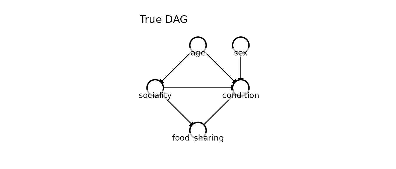

Causal Discovery

Before estimating effects, researchers often want to verify their causal graph against alternative hypotheses.

Suppose a reviewer suggests two alternative models: 1. Alt1: Sociality has no measured cause - the apparent age → sociality link is just noise. 2. Alt2: Body condition causes sociality (healthier individuals have more energy to socialize).

dag_alt1 <- list(
  age          = c(),
  sex          = c(),
  sociality    = c(),
  food_sharing = "sociality",
  condition    = c("age", "sex", "sociality", "food_sharing")
)

dag_alt2 <- list(
  age          = c(),
  sex          = c(),
  condition    = c("age", "sex"),
  food_sharing = "condition",
  sociality    = c("age", "food_sharing", "condition")
)

library(patchwork)
kagu_plot_dag(dag_alt1, node_pos) + ggtitle("Alt1: Sociality has no cause") +
kagu_plot_dag(dag_alt2, node_pos) + ggtitle("Alt2: Condition -> Sociality")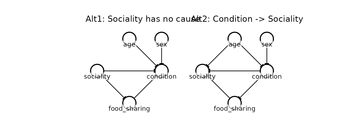

We can use Kagu’s causal discovery engine to score our theoretically proposed DAG against these alternatives. Kagu evaluates the full joint marginal likelihood of the non-linear Gaussian Process fits.

# Pass the specific DAGs to discover over. Naming them means the summary table
# refers to each structure by name; unnamed DAGs get ids "A", "B", "C", ... and
# can be inspected with res$get_dag(id) / res$plot_dag(id).
res <- KaguModel$discover(
  df,
  dags = list("True" = dag_true, "Alt 1" = dag_alt1, "Alt 2" = dag_alt2)
)
res$summary()
#> # A tibble: 3 × 5
#>    rank id    n_edges log_marglik posterior_prob
#>   <int> <chr>   <int>       <dbl>          <dbl>
#> 1     1 True        6       -296.       8.34e- 1
#> 2     2 Alt 1       5       -298.       1.66e- 1
#> 3     3 Alt 2       6       -335.       7.10e-18

Kagu places most of the posterior (~83%) on dag_true, but crucially it does not claim certainty. Alt2 - the hypothesis that body condition causes sociality - is decisively rejected (~0%): reversing those edges contradicts the strong, non-linear signature that sex, sociality and food_sharing jointly leave in condition. But Alt1, which drops the single age → sociality edge (claiming sociality has no measured cause), still retains ~17% of the posterior. With only 50 noisy individuals the weak influence of age on sociality is genuinely hard to detect, and Kagu reports that ambiguity honestly rather than papering over it.

Two things are worth noting. First, the parents of condition are pinned down with near-certainty across every competitive structure - the strong sex * sociality interaction gives the GP a non-linear signature that no reversal of those edges can mimic. Second, the posterior-over-DAGs framing carries the residual structural uncertainty forward rather than discarding it, so we can go on to estimate effects while remaining appropriately humble about which structure generated the data.

The Table II Fallacy

Now that we are confident in our DAG, we want to answer our primary research question: Does sociality improve body condition?

A classic (but flawed) approach in ecology is to fit a single multiple regression model including all measured variables, and read the coefficients from the resulting table (the so-called “Table II”).

summary(lm(condition ~ sociality + food_sharing + age + sex, data = df))$coefficients
#>                 Estimate Std. Error   t value     Pr(>|t|)
#> (Intercept)   0.08223808  0.2111311  0.389512 6.987348e-01
#> sociality    -0.39387054  0.1786109 -2.205188 3.259281e-02
#> food_sharing  0.82683458  0.1659337  4.982921 9.737184e-06
#> age           0.32573026  0.2352380  1.384684 1.729768e-01
#> sex           0.35112375  0.2108787  1.665051 1.028510e-01

Looking at this table, a researcher would incorrectly conclude: 1. Sociality is bad for condition: its coefficient is negative and statistically significant ( $p \approx 0.03$ ). 2. The only beneficial pathway is food sharing.

Both conclusions are wrong. This is the Table II Fallacy. By including food_sharing (a mediator) in the model, the coefficient for sociality is stripped of its positive indirect effect. What remains is the direct effect - strongly positive for females, strongly negative for males - and, with no sex * sociality interaction term in the model, the linear fit collapses those opposing slopes into a single misleading number. Here it lands significantly negative, exactly inverting sociality’s true (large, positive) effect for half the population.

Estimating the true effects with Kagu

Let’s fit our validated DAG using Kagu.

mod <- KaguModel$new(dag_true)
mod$fit(df)

If we ask Kagu for the total marginal effect of sociality on condition, it automatically handles the confounding by age and integrates out the downstream mediator food_sharing correctly via Do-calculus.

# The average total effect of a 1-unit increase in sociality
mod$effects("sociality", "condition", hdi = 0.95)$summary()
#> # A tibble: 1 × 8
#>   source    target       from    to  mean    sd hdi_lower hdi_upper
#>   <chr>     <chr>       <dbl> <dbl> <dbl> <dbl>     <dbl>     <dbl>
#> 1 sociality condition -0.0910 0.909 0.384 0.231   -0.0603     0.844

The point estimate is modestly positive (~0.38), but the 95% HDI is very wide and straddles zero. This is not a failure - it is Kagu being honest. The population-averaged total effect is pulled in two directions at once: the food-sharing mediation contributes a positive push, while the direct effect of sociality is strongly positive in females and strongly negative in males, so on average it nearly cancels and mostly inflates the spread. A single population-averaged number is therefore almost meaningless here; the wide HDI is Kagu’s way of telling us the effect is highly heterogeneous across the population. In the next section we split it apart by sex to reveal exactly what that average conceals.

Examining the mediator

We can also easily query multiple different effects from the same fitted model. For instance, what is the direct effect of our mediator, food sharing?

mod$effects("food_sharing", "condition", hdi = 0.95)$summary()
#> # A tibble: 1 × 8
#>   source       target      from    to  mean     sd hdi_lower hdi_upper
#>   <chr>        <chr>      <dbl> <dbl> <dbl>  <dbl>     <dbl>     <dbl>
#> 1 food_sharing condition -0.194 0.806 0.854 0.0920     0.692      1.05
mod$effects("food_sharing", "condition", sweep = TRUE, hdi = 0.95)$plot() +
  ggtitle("Direct effect of Food Sharing on Condition")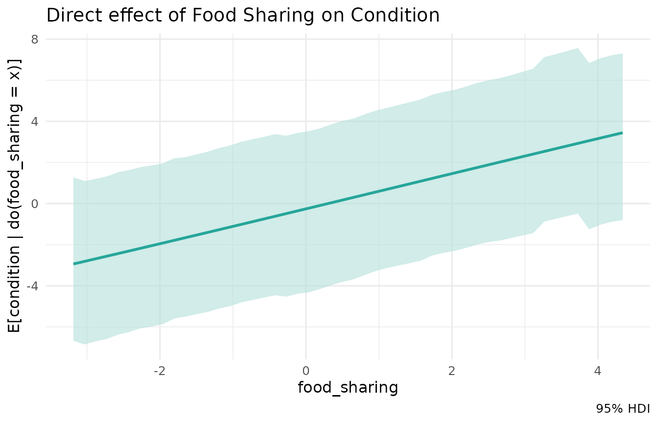

The model recovers the direct effect of food sharing ( $\approx 0.85$ here - close to the true value of 0.8, correctly identified as the strongest single pathway, and the one coefficient the flawed linear table got roughly right!).

Unmasking the interaction

Because Kagu models each node as a Gaussian Process, it has already learned the sex * sociality interaction automatically. We can visualise the true, divergent effects of sociality by using a sweep and passing a list of conditions.

eff_multi <- mod$effects(
  source = "sociality",
  target = "condition",
  sweep = TRUE,
  hdi = 0.95,
  # Sweep over the well-supported central range (sociality has sd ~1.5); going
  # far into the sparse tails just shows the GP reverting to its prior.
  sweep_range = c(-2, 2),
  conditions = list(
    list(sex = -1), # Females
    list(sex =  1)  # Males
  )
)

eff_multi$plot() +
  scale_color_manual(values = c("sex=-1" = "#ff7043", "sex=1" = "#26a69a"),
                     labels = c("Female", "Male")) +
  scale_fill_manual(values = c("sex=-1" = "#ff7043", "sex=1" = "#26a69a"),
                    labels = c("Female", "Male")) +
  labs(
    title = "The true total effect of Sociality on Body Condition",
    subtitle = "Opposing direct effects are automatically unmasked by the GP",
    x = "Intervention: do(Sociality)",
    y = "Expected Body Condition",
    color = "Sex", fill = "Sex"
  )

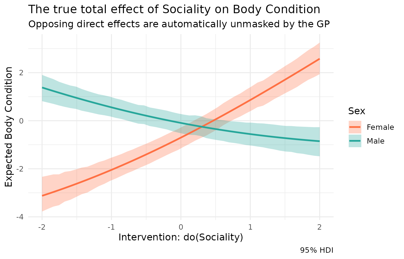
The diverging plot reveals exactly what the classic regression table hid: sociality has a massive effect on body condition for both sexes. For females, the stress-buffering benefits of sociality compound with the food-sharing benefits, resulting in a steep positive slope. For males, the costs of agonistic competition overwhelm the food-sharing benefits, resulting in a negative slope.

We can read off the same story quantitatively by querying the conditional (per-sex) total effect directly:

mod$effects("sociality", "condition", conditions = list(sex = -1), hdi = 0.95)$summary()  # Females
#> # A tibble: 1 × 8
#>   source    target       from    to  mean    sd hdi_lower hdi_upper
#>   <chr>     <chr>       <dbl> <dbl> <dbl> <dbl>     <dbl>     <dbl>
#> 1 sociality condition -0.0910 0.909  1.44 0.142      1.16      1.71
mod$effects("sociality", "condition", conditions = list(sex =  1), hdi = 0.95)$summary()  # Males
#> # A tibble: 1 × 8
#>   source    target       from    to   mean    sd hdi_lower hdi_upper
#>   <chr>     <chr>       <dbl> <dbl>  <dbl> <dbl>     <dbl>     <dbl>
#> 1 sociality condition -0.0910 0.909 -0.572 0.121    -0.789    -0.329

For females the effect is strongly positive ( $\approx 1.4$ ), for males strongly negative ( $\approx -0.6$ ) - two large, opposing effects that the population-averaged estimate above (and the linear regression table) washed out to near zero.

Why classic model selection fails

To drive this point home, let’s see what happens if a researcher realizes their basic linear model was inadequate and attempts to rely purely on data-driven model selection (like step-wise AIC) to find the “best” model for condition.

# Try all possible main effects and 2-way interactions
full_model <- lm(condition ~ (age + sex + sociality + food_sharing)^2, data = df)

# Use step-wise AIC to find the best model
best_lm <- step(full_model, trace = FALSE)

summary(best_lm)$coefficients
#>                           Estimate Std. Error    t value     Pr(>|t|)
#> (Intercept)            -0.10518871 0.06828718  -1.540387 1.307935e-01
#> age                     0.60368934 0.06888731   8.763433 4.044857e-11
#> sex                     0.29804661 0.06231479   4.782920 2.054145e-05
#> sociality              -0.05597326 0.05490741  -1.019412 3.137090e-01
#> food_sharing            0.82411489 0.04782411  17.232205 6.380261e-21
#> sex:sociality          -1.02705168 0.04593807 -22.357312 2.653017e-25
#> sociality:food_sharing  0.05055655 0.01948286   2.594925 1.288911e-02

Even though the AIC algorithm successfully detected the strong sex:sociality interaction and correctly rejected the simpler linear models, the coefficients from this “best” model are deeply misleading for causal inference:

Because food_sharing (the mediator) was retained as a predictor by the AIC algorithm, the base sociality coefficient ( $\approx -0.06$ ) is entirely stripped of its indirect pathway.
If the researcher takes the food_sharing coefficient ( $\approx 0.82$ ) and treats it as the causal effect of food sharing, they are committing the Table II Fallacy. The variables chosen by AIC to optimally predict condition are fundamentally not the correct adjustment set for estimating the causal effect of food_sharing.

Kagu avoids all of this by explicitly separating the causal structure (the DAG) from the functional form (the GPs). It discovers the interactions automatically to identify the structure, and then rigorously applies Do-calculus to estimate the exact marginal or conditional effects without falling into the Table II trap!