Causal structure discovery

The other vignettes take the DAG as given. But the DAG is itself a hypothesis about how a system works, and often it is exactly what we want to learn. Kagu can treat structure discovery as Bayesian inference over graphs: fit a GCM to every candidate DAG, and turn the marginal likelihoods into a posterior distribution over structures,

$$P(G \mid X) \;\propto\; P(X \mid G)\, P(G).$$

Here $P(X \mid G)$ is the marginal likelihood of the data under graph $G$ (computed in closed form from the per-node Gaussian-process fits) and $P(G)$ is a prior over structures (currently uniform). Rather than returning a single “best” graph, this returns a full probability distribution - an honest representation of what the data can and cannot tell us about causal structure.

A worked example

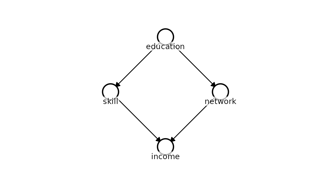
We simulate a four-variable system with a known structure. education is a root cause of both skill and network; income is driven by skill and network. There is no direct education → income edge, and skill and network are not directly linked.

true_dag <- list(
  education = c(),
  skill     = "education",
  network   = "education",
  income    = c("skill", "network")
)

kagu_plot_dag(true_dag, node_pos = list(
  education = c(0,  0),
  skill     = c(1, -1),
  network   = c(1,  1),
  income    = c(2,  0)
))

n         <- 50
education <- rnorm(n)
skill     <- 0.8 * education + rnorm(n, sd = 0.6)
network   <- 0.6 * education + rnorm(n, sd = 0.6)
income    <- 1.0 * skill + 0.7 * network + rnorm(n, sd = 0.6)

df <- data.frame(education, skill, network, income)

Running the search

The number of DAGs grows explosively with the number of variables, so we narrow the space with background knowledge. Here we know only that education comes first - nothing causes a person’s education in this system - so we use disallowed to forbid any edge pointing into education. The ordering among skill, network, and income is left for the data to resolve. This is exactly the kind of light domain knowledge a researcher can bring to a problem.

disallowed <- list(
  c("skill",   "education"), 
  c("network", "education"), 
  c("income", "education")
)

result <- KaguModel$discover(df, disallowed = disallowed)

result
#> <DiscoveryResult: 199 DAGs, 25 unique local fits>
#> # A tibble: 5 × 5
#>    rank id    n_edges log_marglik posterior_prob
#>   <int> <chr>   <int>       <dbl>          <dbl>
#> 1     1 GK          5       -191.          0.164
#> 2     2 GQ          6       -191.          0.162
#> 3     3 GM          6       -191.          0.162
#> 4     4 FY          4       -191.          0.143
#> 5     5 GE          5       -191.          0.141

The search evaluated every DAG consistent with that constraint, but - thanks to the Markov factorisation - only had to fit each unique node ~ parents model once (far fewer fits than DAGs).

Tighter constraints: required edges

For larger systems, the number of candidate DAGs can easily exceed Kagu’s safety limits (capped at $2^{24}$ subsets, roughly 5 unconstrained nodes). If you have stronger structural beliefs-such as an edge that absolutely must exist-you can pass required. This shrinks the search space dramatically by removing those edges from the combinatorics.

# Suppose we know education -> skill and education -> network are certain
result_req <- KaguModel$discover(
  df, 
  disallowed = disallowed, 
  required = list(c("education", "skill"), c("education", "network"))
)

Explicit DAG comparison: dags

Sometimes you don’t want to search the whole graph space. If you have a few specific, theoretically motivated hypotheses, you can pass them directly via dags. Kagu will skip the combinatorial search entirely and just compute the posterior probabilities over your explicit models.

dag_mediation <- list(education = c(), skill = "education", income = "skill")
dag_direct    <- list(education = c(), skill = c(), income = "education")

result_explicit <- KaguModel$discover(df, dags = list(dag_mediation, dag_direct))

The posterior over DAGs

$summary() ranks the structures by posterior probability. Each row is a whole DAG, referenced by a short id (here the enumerated graphs get ids "A", "B", "C", …; had we passed a named list of DAGs, those names would be used instead). posterior_prob is $P(G \mid X)$.

result$summary()
#> # A tibble: 10 × 5
#>     rank id    n_edges log_marglik posterior_prob
#>    <int> <chr>   <int>       <dbl>          <dbl>
#>  1     1 GK          5       -191.        0.164  
#>  2     2 GQ          6       -191.        0.162  
#>  3     3 GM          6       -191.        0.162  
#>  4     4 FY          4       -191.        0.143  
#>  5     5 GE          5       -191.        0.141  
#>  6     6 GA          5       -191.        0.141  
#>  7     7 FO          6       -193.        0.0355 
#>  8     8 CI          6       -194.        0.0160 
#>  9     9 CQ          6       -195.        0.00645
#> 10    10 FM          5       -195.        0.00635

To see what a given structure actually is, look it up by its id with result$get_dag(id), or plot it directly:

top_id <- result$summary()$id[1]
result$plot_dag(top_id)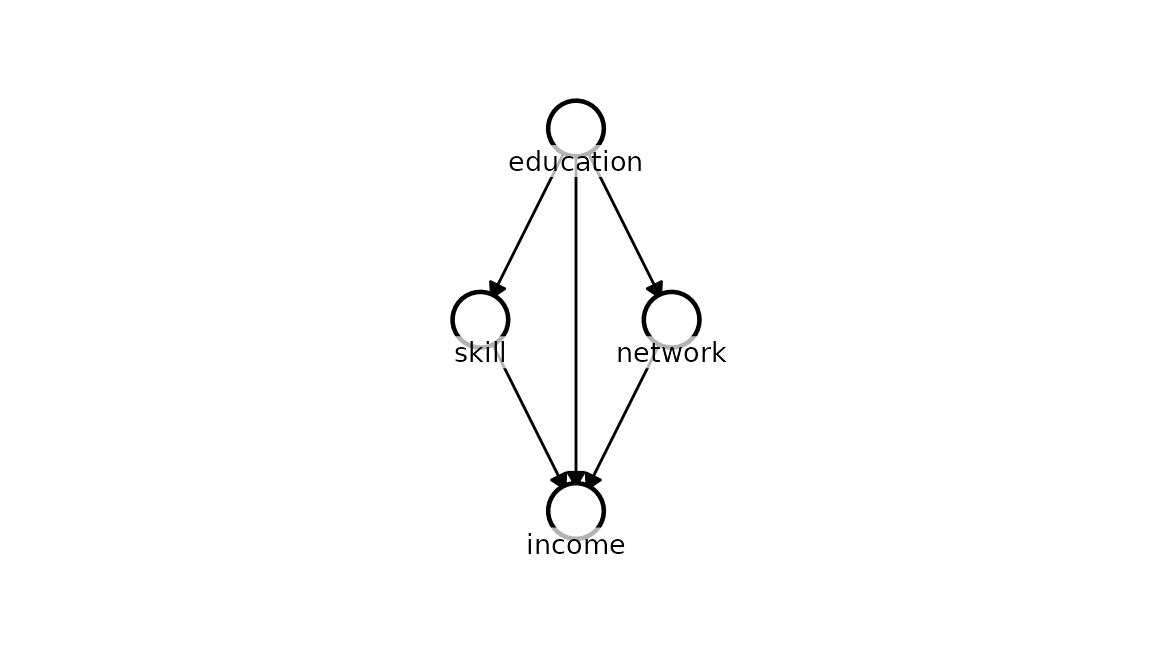

No single DAG runs away with the posterior - the top few structures each hold only around a sixth of the mass. That is not a defect: with a handful of variables and this much noise, the data simply cannot single out one graph. What it can do is concentrate the mass onto a small cluster of closely-related structures that all agree on the important causal edges, and rule the rest out. We can’t always name the one true DAG, but we can zoom in on the handful that matter.

The histogram makes the shape of the posterior clear. With the true data-generating DAG highlighted, we can see how much of the probability mass it captures.

result$plot(true_dag = true_dag)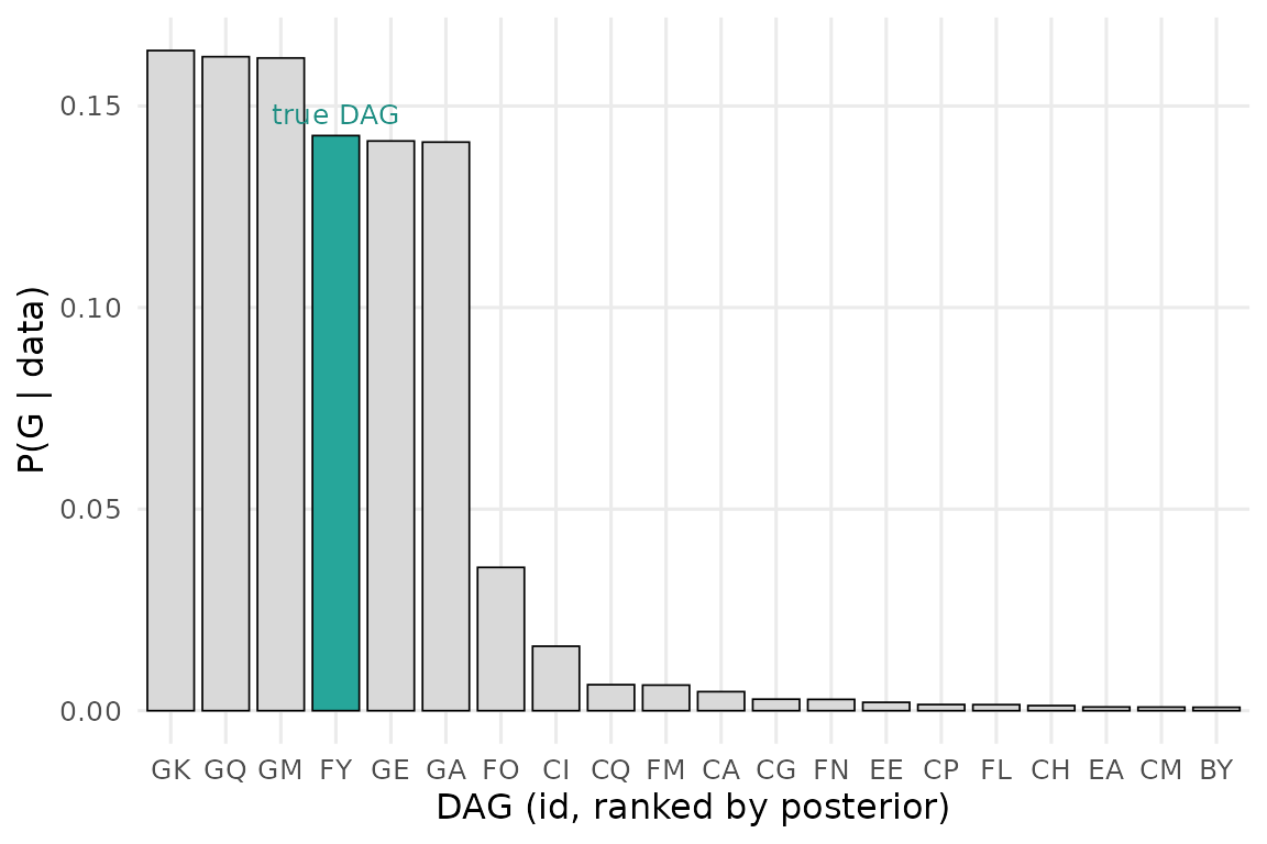

Edge probabilities

Often we care less about the single best graph than about specific causal questions - does this edge exist, and in which direction? $edge_probabilities() marginalises over the whole posterior to give the probability of each directed edge, $P(\text{from} \to \text{to} \mid X) = \sum_{G \ni \text{edge}} P(G \mid X)$.

result$edge_probabilities()
#> # A tibble: 9 × 3
#>   from      to        prob
#>   <chr>     <chr>    <dbl>
#> 1 education network 0.992 
#> 2 education skill   0.991 
#> 3 network   income  0.959 
#> 4 skill     income  0.917 
#> 5 education income  0.575 
#> 6 network   skill   0.365 
#> 7 skill     network 0.315 
#> 8 income    skill   0.0834
#> 9 income    network 0.0396

This is where the posterior becomes genuinely useful. The four true edges (education→skill, education→network, skill→income, network→income) each carry almost all of the probability - the data is confident they exist and point the way they do - and the clearest edge reversals are correctly assigned low probability. What lingers is a redundant direct education→income edge: even though education’s effect on income is fully mediated by skill and network, observational data at this sample size cannot completely exclude a direct path, so that edge keeps a moderate probability rather than collapsing to zero. Kagu reports the residual ambiguity honestly instead of pretending the edge is ruled out.

Effects under structural uncertainty

When the structure is uncertain, committing to a single DAG - even the most probable one - throws away that uncertainty. Instead, query the effect directly on the DiscoveryResult: it averages over the entire posterior of DAGs, weighting each by $P(G \mid X)$, $$P(Q \mid X) = \sum_G P(Q \mid X, G)\, P(G \mid X).$$ The call signature and the returned object are exactly those of the single-DAG model$effects(), so everything downstream - summaries, plots - works the same.

result$effects("education", "income")$summary()
#> # A tibble: 1 × 8
#>   source    target    from    to  mean    sd hdi_lower hdi_upper
#>   <chr>     <chr>    <dbl> <dbl> <dbl> <dbl>     <dbl>     <dbl>
#> 1 education income -0.0357 0.964  1.64 0.385     0.983      2.24

This estimate carries both the parameter uncertainty within each model and the structural uncertainty between models. DAGs in which education has no causal path to income simply contribute a zero effect, exactly as they should.

The limits of observational data

Structure discovery is powerful, but it cannot manufacture information the data do not contain - and a good method should tell you so. A classic example is a three-variable system with linear relationships. Suppose x causes y, which in turn causes z:

n <- 500
x <- rnorm(n)
y <- 0.8 * x + rnorm(n, sd = 0.5)
z <- 0.8 * y + rnorm(n, sd = 0.5)

res_linear <- KaguModel$discover(data.frame(x, y, z))
head(res_linear$summary())
#> # A tibble: 6 × 5
#>    rank id    n_edges log_marglik posterior_prob
#>   <int> <chr>   <int>       <dbl>          <dbl>
#> 1     1 G           2      -1526.         0.324 
#> 2     2 I           3      -1526.         0.248 
#> 3     3 R           2      -1527.         0.100 
#> 4     4 T           3      -1527.         0.0769
#> 5     5 U           2      -1527.         0.0705
#> 6     6 W           3      -1527.         0.0679

The search decisively rejects the independent graph and any structure that violates the data’s conditional independencies, but it does not collapse onto a single winner. Instead the mass is shared across a cluster of closely-related graphs: the reverse chain (y → x; z → y), the fork (y → x; y → z), and the true forward chain (x → y; y → z) - plus versions of each carrying one redundant extra edge that the data cannot rule out.

And it is right to spread out. In a linear system, the three chains imply the identical observational distribution (they are Markov equivalent). They all encode that x and z are independent given y, and no quantity of purely observational linear data can distinguish them - nor can it exclude a weak extra edge that adds nothing to the fit. Reporting this uncertainty honestly, rather than picking an arbitrary winner, is exactly what makes the posterior-over-DAGs framing trustworthy.

(Note that strict Markov equivalence often relies on linear-Gaussian assumptions. If the underlying relationships were non-linear, Kagu’s Gaussian-process mechanisms could often uniquely identify the exact true structure from observational data alone!)

Breaking the tie requires stepping outside passive linear observation: non-linear relationships, temporal ordering or domain knowledge (as in the worked example above), or an intervention - randomising x and seeing whether y and z respond.

The uniform prior used here can, in future, be replaced by priors that favour sparsity or encode softer structural beliefs - the posterior machinery is unchanged.